SFEM is a C++ framework for the solution of Partial Differential Equations on unstructured meshes, using the Finite Element and Finite Volume methods. It supports distributed memory parallelism via the MPI protocol. SFEM utilizes METIS for mesh partitioning, and, optionally, PETSc and SLEPc can be used for solving linear and eigenproblems respectively. However, an iterative linear solver suite is also included natively with SFEM.

Below are a few examples detailing the current capabilities of SFEM. The code for these examples will be added soon.

FEM examples:

• Spherial shell under internal pressure
• Potential flow
• Modal analysis

FVM examples:

• 2D Riemann Problem
• Nonlinear Heat Equation

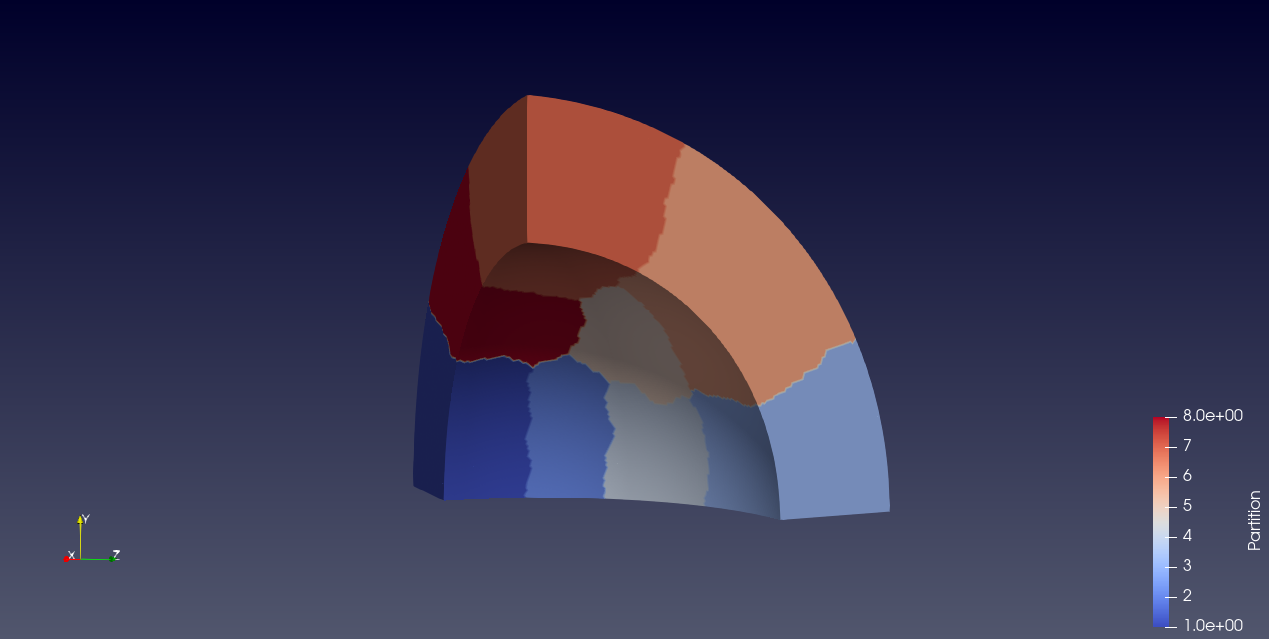
Spherical Shell under Internal Pressure

This example highlights SFEM’s parallelization capabilities. A spherical shell octant is meshed with ~770,000 second order tetrahedral elements, corresponding to approximately 1.5 million degrees of freedom. The shell is considered linear elastic and is subject to a costant pressure value acting on its inner wall. The mesh is partitioned among 8 MPI processes using METIS and the resulting linear system is solved by PETSc’s Conjugate Gradient solver.

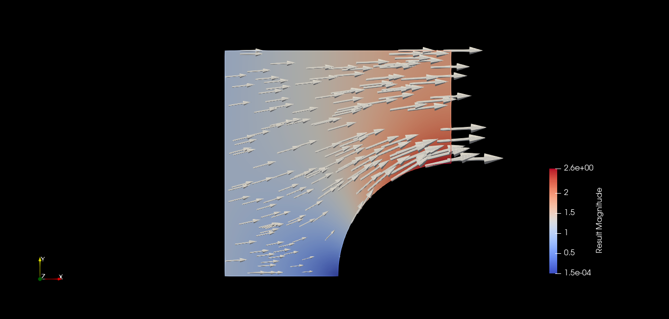
Potential Flow

In this example SFEM is used to solve a potential flow problem around a quarter circle. The problem is discretized using third-order quadrilateral elements, and a Laplace equation is solved for the velocity potential. The velocity field, defined as the gradient of the potential, is then projected onto the same Continuous Galerkin space using a L2 projection.

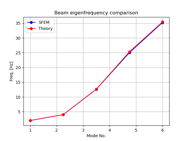
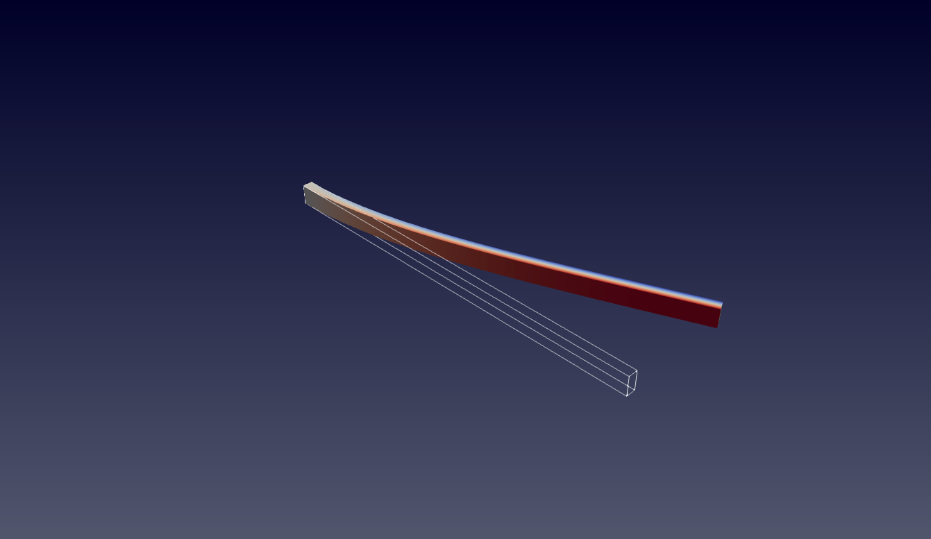
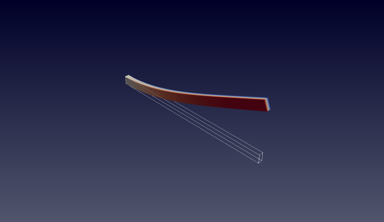
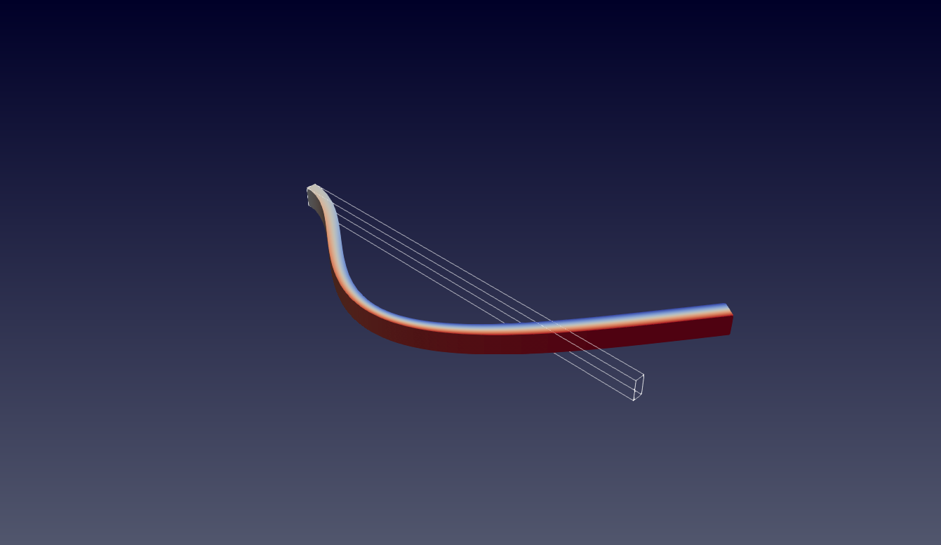
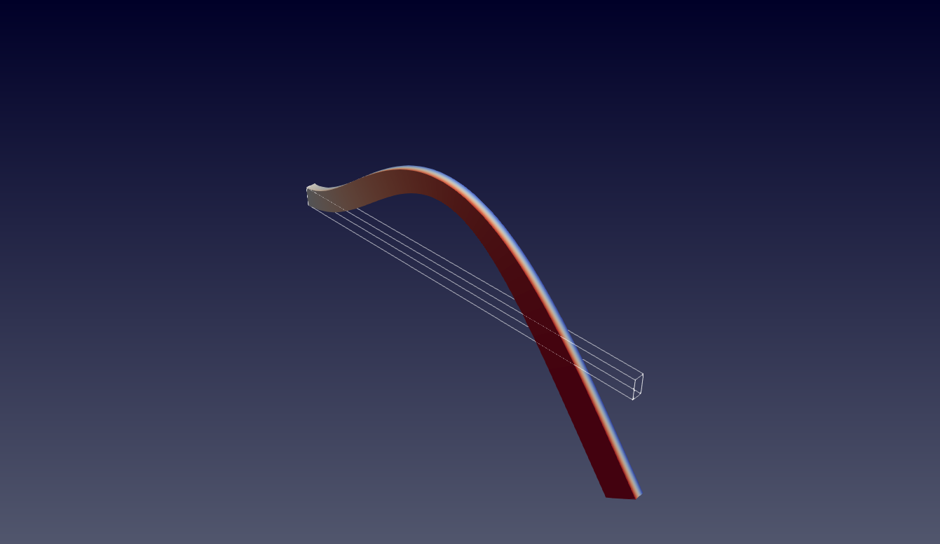
Beam Modal Analysis

In this example SFEM is used to compute the first six eigenmodes of an elastic beam, which is fully fixed on one end. The beam is discretized using second-order tetrahedral elements and the resulting eigenproblem is solved using SLEPc. For validation, the resulting frequencies are compared with those provided by beam theory.

Beam Modal Analysis: Plots of the first four modes

2D Riemann Problem

This example solves the two-dimensional Euler equations with piecewise-constant initial data in a rectangular domain. The domain is split into four quadrants, each having different initial density and pressure values. A conservative, piecewise linear finite-volume method is used, combined with the HLLC approximate Riemann problem solver. The discretized equations are evolved in time using a second-order Runge-Kutta integrator. A uniform mesh of 2056 cells in each direction is used, and the program is executed with 32 MPI processes.

Nonlinear Heat Equation

This example solves the heat equation in three dimensions, with temperature dependent coefficients and a Gaussian heat source. The finite-volume method is used for discretization, and the transient problem is solved implicitly using SFEM’s native Conjugate Gradient solver. A uniform mesh of size 64x64x8 is used, and the program is executed with 4 MPI processes. This is essentially the same physical problem solved by WELDSIM .